# Example Code for the Optimum Filters

Import qetpy and other necessary packages.

import numpy as np
import matplotlib.pyplot as plt
import qetpy as qp
from pprint import pprint

Use QETpy to generate some simulated TES noise

We can use qetpy.sim.TESnoise to help create a simulated PSD with characteristic TES parameters.

fs = 625e3
f = np.fft.fftfreq(32768, d=1/fs)
noisesim = qp.sim.TESnoise(r0=0.03)
psd_sim = noisesim.s_iload(freqs=f) + noisesim.s_ites(freqs=f) + noisesim.s_itfn(freqs=f)

f_fold, psd_sim_fold = qp.foldpsd(psd_sim, fs=fs)

fig, ax = plt.subplots(figsize=(8, 6))
ax.loglog(f_fold, psd_sim_fold**0.5, color="blue", alpha=0.5, label="Simulated PSD, No Spikes")
ax.set_ylim(1e-12,1e-9)
ax.grid()
ax.grid(which="minor", linestyle="dotted")
ax.tick_params(which="both", direction="in", right=True, top=True)
ax.legend(loc="best")
ax.set_title("Simulated Current PSD")
ax.set_ylabel("PSD [A/$\sqrt{\mathrm{Hz}}$]")
ax.set_xlabel("Frequency [Hz]")
fig.tight_layout()

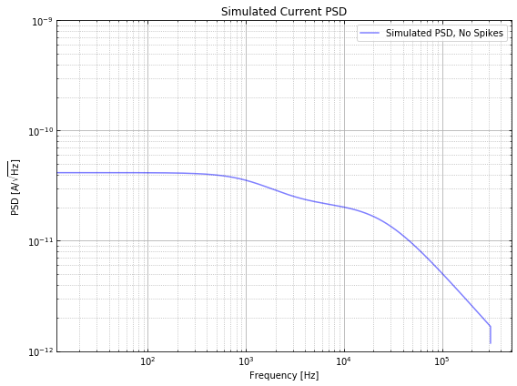
With a PSD, we can use qetpy.gen_noise to generate random noise from the PSD (assuming the frequencies are uncorrelated). Then, we will create an example pulse.

# create a template
pulse_amp = 1e-6 # [A]
tau_f = 66e-6 # [s]
tau_r = 20e-6 # [s]

t = np.arange(len(psd_sim))/fs

pulse = np.exp(-t/tau_f)-np.exp(-t/tau_r)
pulse_shifted = np.roll(pulse, len(t)//2)
template = pulse_shifted/pulse_shifted.max()

# use the PSD to create an example trace to fit
noise = qp.gen_noise(psd_sim, fs=fs, ntraces=1)[0]
signal = noise + np.roll(template, 100)*pulse_amp # note the shift we have added, 160 us

Fit a single pulse with OptimumFilter

With a pulse created, let’s use the qetpy.OptimumFilter class to run different Optimum Filters.

qp.OptimumFilter?

Below, we print the different methods available in qetpy.OptimumFilter. In this notebook, we will demo the ofamp_nodelay, ofamp_withdelay, ofamp_pileup_iterative, and update_signal methods. It is highly recommend to read the documentation for the other methods, as there are many useful ones!

method_list = sorted([func for func in dir(qp.OptimumFilter) if callable(getattr(qp.OptimumFilter, func)) and not func.startswith("__")])
pprint(method_list)

['chi2_lowfreq',
 'chi2_nopulse',
 'energy_resolution',
 'ofamp_baseline',
 'ofamp_nodelay',
 'ofamp_pileup_iterative',
 'ofamp_pileup_stationary',
 'ofamp_withdelay',
 'time_resolution',
 'update_signal']

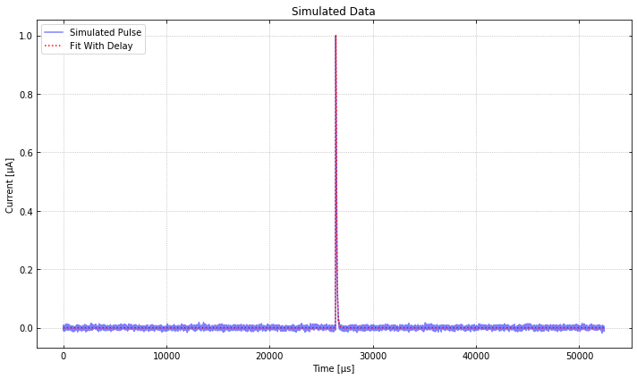
Let’s run the Optimum Filter without and with a time-shifting degree of freedom.

OF = qp.OptimumFilter(signal, template, psd_sim, fs) # initialize the OptimumFilter class
amp_nodelay, chi2_nodelay = OF.ofamp_nodelay()
amp_withdelay, t0_withdelay, chi2_withdelay = OF.ofamp_withdelay()

print(f"No Delay Fit: amp = {amp_nodelay*1e6:.2f} μA, χ^2 = {chi2_nodelay:.2f}")
print(f"With Delay Fit: amp = {amp_withdelay*1e6:.2f} μA, t_0 = {t0_withdelay*1e6} μs, χ^2 = {chi2_withdelay:.2f}")

No Delay Fit: amp = -0.04 μA, χ^2 = 210399.75
With Delay Fit: amp = 1.00 μA, t_0 = 160.0 μs, χ^2 = 32407.30

Since we have added a 160 us shift, we see that the “with delay” optimum filter fit the time-shift perfectly, and the chi-squared is very close to the number of degrees of freedom (32768), as we would expect for a good fit.

fig, ax = plt.subplots(figsize=(10, 6))
ax.plot(t*1e6, signal*1e6, label="Simulated Pulse", color="blue", alpha=0.5)
ax.plot(t*1e6, amp_withdelay*np.roll(template, int(t0_withdelay*fs))*1e6,
        label="Fit With Delay", color="red", linestyle="dotted")
ax.set_ylabel("Current [μA]")
ax.set_xlabel("Time [μs]")
ax.set_title("Simulated Data")
lgd = ax.legend(loc="upper left")
ax.tick_params(which="both", direction="in", right=True, top=True)
ax.grid(linestyle="dotted")
fig.tight_layout()

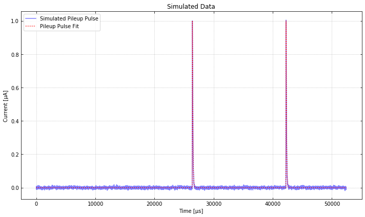
Add a pileup pulse and fit with OptimumFilter

Let’s now add a second (pileup) pulse in order to see how we can use ofamp_pileup_iterative.

pileup = signal + np.roll(template, 10000)*pulse_amp

OF.update_signal(pileup) # update the signal in order to fit a new trace
amp_withdelay, t0_withdelay, chi2_withdelay = OF.ofamp_withdelay(nconstrain=300)
amp_pileup, t0_pileup, chi2_pileup = OF.ofamp_pileup_iterative(amp_withdelay, t0_withdelay)

print(f"With Delay Fit: amp = {amp_withdelay*1e6:.2f} μA, t_0 = {t0_withdelay*1e6} μs, χ^2 = {chi2_withdelay:.2f}")
print(f"Pileup Fit: amp = {amp_pileup*1e6:.2f} μA, t_0 = {t0_pileup*1e6} μs, χ^2 = {chi2_pileup:.2f}")

With Delay Fit: amp = 1.00 μA, t_0 = 160.0 μs, χ^2 = 209503.04
Pileup Fit: amp = 1.00 μA, t_0 = 16000.0 μs, χ^2 = 32407.28

As expected, the pileup optimum filter fit the data very well, as we can see from the chi-squared above.

fig, ax = plt.subplots(figsize=(10, 6))

ax.plot(t*1e6, pileup*1e6, label="Simulated Pileup Pulse", color="blue", alpha=0.5)
ax.plot(t*1e6, amp_withdelay*np.roll(template, int(t0_withdelay*fs))*1e6 + \
        amp_pileup*np.roll(template, int(t0_pileup*fs))*1e6,
        label="Pileup Pulse Fit", color="red", linestyle="dotted")

ax.set_ylabel("Current [μA]")
ax.set_xlabel("Time [μs]")
ax.set_title("Simulated Data")
lgd = ax.legend(loc="upper left")
ax.tick_params(which="both", direction="in", right=True, top=True)
ax.grid(linestyle="dotted")
fig.tight_layout()

Nonlinear Fitting

What about when we do not have a template? The qetpy.OFnonlin class has been written to fit the fall times as well, which is useful for cases where we do not have a template, or we know that the template will not match the data well.

pulse_amp = 1e-6
tau_f = 160e-6
tau_r = 20e-6

t = np.arange(len(psd_sim))/fs

pulse = np.exp(-t/tau_f)-np.exp(-t/tau_r)
pulse_shifted = np.roll(pulse, len(t)//2)
template = pulse_shifted/pulse_shifted.max()

noise = qp.gen_noise(psd_sim, fs=fs, ntraces=1)[0]
signal = noise + np.roll(template, 100)*pulse_amp

We can try using our “bad” template (with a 66 us fall time), but we will see that the chi-squared indicates a non-ideal fit.

OF.update_signal(signal) # update the signal in order to fit a new trace
amp_withdelay, t0_withdelay, chi2_withdelay = OF.ofamp_withdelay(nconstrain=300)

print(f"With Delay Fit: amp = {amp_withdelay*1e6:.2f} μA, t_0 = {t0_withdelay*1e6:.2f} μs, χ^2 = {chi2_withdelay:.2f}")

With Delay Fit: amp = 1.07 μA, t_0 = 163.20 μs, χ^2 = 72524.20

Let’s use qetpy.OFnonlin to do the fit. To help visualize the fit, we will use the parameter lgcplot=True to plot the fit in frequency domain and time domain

qp.OFnonlin?

qp.OFnonlin.fit_falltimes?

nonlinof = qp.OFnonlin(psd_sim, fs, template=None)
params, error, _, chi2_nonlin, success = nonlinof.fit_falltimes(signal, npolefit=2, lgcfullrtn=True, lgcplot=True)

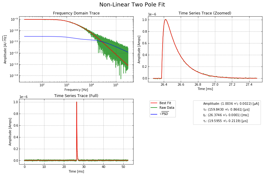
print(f"Nonlinear fit: χ^2 = {chi2_nonlin * (len(nonlinof.data)-nonlinof.dof):.2f}")

Nonlinear fit: χ^2 = 32719.95

And we see that the fit using qetpy.OFnonlin is great! The chi-squared is near the number of degrees of freedom (32768), which indicates that we have a good fit.

For further documentation on the different fitting functions, please visit https://qetpy.readthedocs.io/en/latest/qetpy.core.html#module-qetpy.core._fitting.