Using the autocuts and IterCut Algorithms
This is a quick look at how to use the autocuts and the IterCut
algorithms. The autocuts function acts as a black box (the user
cannot see what is going on under the hood), while IterCut allows
the user to understand each cut being applied to data. For quick
results, autocuts is usually sufficient, but IterCut is very
useful to actually understand what is happening.
Note that there are many more optional arguments than what are shown here in the notebook. As always, we recommend reading the docstrings!
First, let’s import our functions.
import numpy as np
import matplotlib.pyplot as plt
from qetpy import autocuts, calc_psd, IterCut

# ensure that the notebook is repeatable by using the same random seed
np.random.seed(1)
Now, let’s load the data.
pathtodata = "test_autocuts_data.npy"
traces = np.load(pathtodata)
fs = 625e3
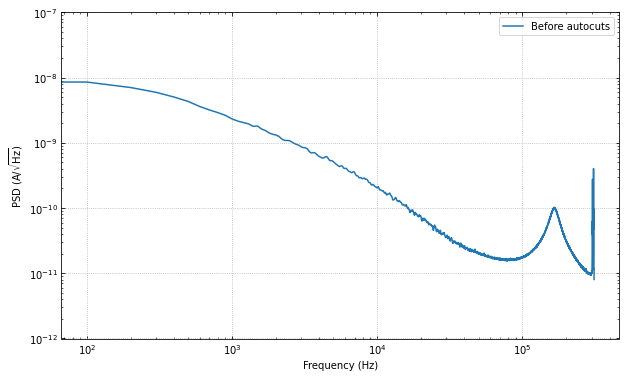
Let’s look at the PSD before the cuts, to get a sense of the change.
f, psd = calc_psd(traces, fs=fs, folded_over=True)
fig, ax = plt.subplots(figsize=(10,6))
ax.loglog(f, np.sqrt(psd), label="Before autocuts")
ax.set_ylim([1e-12,1e-7])
ax.set_xlabel('Frequency (Hz)')
ax.set_ylabel(r'PSD (A/$\sqrt{\mathrm{Hz}}$)')
ax.legend(loc="upper right")
ax.grid(linestyle='dotted')
ax.tick_params(which='both',direction='in',right=True,top=True)
Using autocuts
Apply the autocuts function.
?autocuts
Function to automatically cut out bad traces based on the optimum
filter amplitude, slope, baseline, and chi^2 of the traces.

Parameters
----------
traces : ndarray
    2-dimensional array of traces to do cuts on
fs : float, optional
    Sample rate that the data was taken at
is_didv : bool, optional
    Boolean flag on whether or not the trace is a dIdV curve
outlieralgo : string, optional
    Which outlier algorithm to use. If set to "removeoutliers",
    uses the removeoutliers algorithm that removes data based on
    the skewness of the dataset. If set to "iterstat", uses the
    iterstat algorithm to remove data based on being outside a
    certain number of standard deviations from the mean. Can also
    be set to astropy's "sigma_clip".
lgcpileup1 : boolean, optional
    Boolean value on whether or not do the pileup1 cut (this is the
    initial pileup cut that is always done whether or not we have
    dIdV data). Default is True.
lgcslope : boolean, optional
    Boolean value on whether or not do the slope cut. Default is
    True.
lgcbaseline : boolean, optional
    Boolean value on whether or not do the baseline cut. Default is
    True.
lgcpileup2 : boolean, optional
    Boolean value on whether or not do the pileup2 cut (this cut is
    only done when is_didv is also True). Default is True.
lgcchi2 : boolean, optional
    Boolean value on whether or not do the chi2 cut. Default is
    True.
nsigpileup1 : float, optional
    If outlieralgo is "iterstat", this can be used to tune the
    number of standard deviations from the mean to cut outliers
    from the data when using iterstat on the optimum filter
    amplitudes. Default is 2.
nsigslope : float, optional
    If outlieralgo is "iterstat", this can be used to tune the
    number of standard deviations from the mean to cut outliers
    from the data when using iterstat on the slopes. Default is 2.
nsigbaseline : float, optional
    If outlieralgo is "iterstat", this can be used to tune the
    number of standard deviations from the mean to cut outliers
    from the data when using iterstat on the baselines. Default is
    2.
nsigpileup2 : float, optional
    If outlieralgo is "iterstat", this can be used to tune the
    number of standard deviations from the mean to cut outliers
    from the data when using iterstat on the optimum filter
    amplitudes after the mean has been subtracted. (only used if
    is_didv is True). Default is 2.
nsigchi2 : float, optional
    This can be used to tune the number of standard deviations
    from the mean to cut outliers from the data when using iterstat
    on the chi^2 values. Default is 3.
**kwargs
    Placeholder kwargs for backwards compatibility.

Returns
-------
ctot : ndarray
    Boolean array giving which indices to keep or throw out based
    on the autocuts algorithm.
cut = autocuts(
    traces,
    fs=fs,
)
print(f"The cut efficiency is {np.sum(cut)/len(traces):.3f}.")
The cut efficiency is 0.428.
Let’s compare the PSD after the cuts, we should see the noise go down by a fair amount.
psd_cut = calc_psd(traces[cut], fs=fs, folded_over=True)[1]
fig, ax = plt.subplots(figsize=(10,6))
ax.loglog(f, np.sqrt(psd), label="Before autocuts")
ax.loglog(f, np.sqrt(psd_cut), label="After autocuts")
ax.set_ylim([1e-12,1e-7])
ax.set_xlabel('Frequency (Hz)')
ax.set_ylabel(r'PSD (A/$\sqrt{\mathrm{Hz}}$)')
ax.legend(loc="upper right")
ax.grid(linestyle='dotted')
ax.tick_params(which='both',direction='in',right=True,top=True)
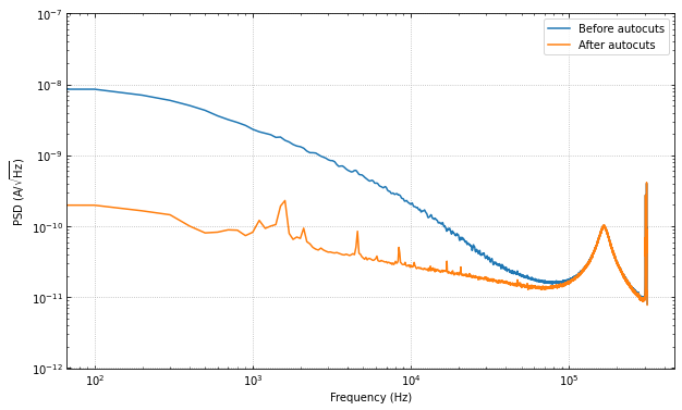
The change is huge! Which makes sense, as we have removed many of the pulses, muon tails, etc. Please note that there may still be “bad” traces in the data, as the autocuts function is not perfect. There may be more cuts that one would like to do that are more specific to the dataset.
Using IterCut for better cut control
A good way of understanding the cuts further than using the black box
that is autocuts is to use the object-oriented version IterCut.
This class allows the user freedom in cut order, which cuts are used,
which algorithms are used for outlier removal, and more.
Below, we match the default parameters and outlier algorithm
(iterstat) to show that the cut efficiency is the same.
IC = IterCut(traces, fs)
IC.pileupcut(cut=2)
IC.slopecut(cut=2)
IC.baselinecut(cut=2)
IC.chi2cut(cut=3)
cut_ic = IC.cmask
print(f"The cut efficiency is {np.sum(cut_ic)/len(traces):.3f}.")
The cut efficiency is 0.428.
psd_cut = calc_psd(traces[cut_ic], fs=fs, folded_over=True)[1]
fig, ax = plt.subplots(figsize=(10,6))
ax.loglog(f, np.sqrt(psd), label="Before IterCut")
ax.loglog(f, np.sqrt(psd_cut), label="After IterCut")
ax.set_ylim([1e-12,1e-7])
ax.set_xlabel('Frequency (Hz)')
ax.set_ylabel(r'PSD (A/$\sqrt{\mathrm{Hz}}$)')
ax.legend(loc="upper right")
ax.grid(linestyle='dotted')
ax.tick_params(which='both',direction='in',right=True,top=True)

With IterCut we can also access the cuts at each step as they have
been iteratively applied, and there is a verbose option for plotting the
passing event and failing events for each cut.
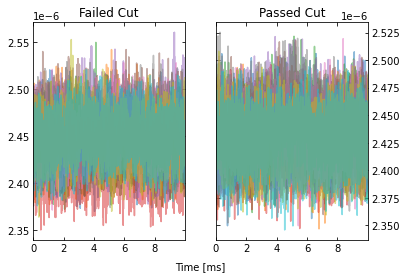
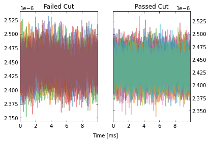
IC = IterCut(traces, fs, plotall=True, nplot=10)
cpileup = IC.pileupcut(cut=2)
cpileup1 = IC.cmask
cslope = IC.slopecut(cut=2)
cbaseline = IC.baselinecut(cut=2)
cchi2 = IC.chi2cut(cut=3)
cut_ic = IC.cmask
This allows to calculate the efficiency of each cut, and we can see what cuts are going the heavy lifting. Note the importance of the denominator being the number of events that passed the previous cuts when calculating these efficiencies. If we were to divide by the number of traces each time, then this would be the total cut efficiency up to that cut. Below, we show the individual performance of each cut.
print(f"The pileup cut efficiency is {np.sum(cpileup)/len(traces):.3f}.")
print(f"The slope cut efficiency is {np.sum(cslope)/np.sum(cpileup):.3f}.")
print(f"The baseline cut efficiency is {np.sum(cbaseline)/np.sum(cslope):.3f}.")
print(f"The chi2 cut efficiency is {np.sum(cchi2)/np.sum(cbaseline):.3f}.")
print("-------------")
print(f"The total cut efficiency is {np.sum(cut_ic)/len(traces):.3f}.")
The pileup cut efficiency is 0.679.
The slope cut efficiency is 0.719.
The baseline cut efficiency is 0.889.
The chi2 cut efficiency is 0.986.
-------------
The total cut efficiency is 0.428.
Thus, we see that the pileup cut is has the lowest efficiency, with the slope cut as a close second. If we were to remove the baseline and chi-squared cuts, then we would expect the PSD to not change noticeably. Let’s test this expectation.
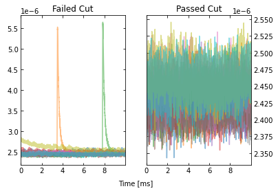
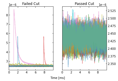
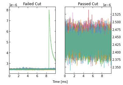
Note that we can also plot the events passing/failing a specific cut by
passing verbose=True, as shown below.
IC = IterCut(traces, fs)
cpileup = IC.pileupcut(cut=2, verbose=True)
cslope = IC.slopecut(cut=2)
cut_ic = IC.cmask
print(f"The pileup cut efficiency is {np.sum(cpileup)/len(traces):.3f}.")
print(f"The slope cut efficiency is {np.sum(cslope)/np.sum(cpileup):.3f}.")
print("-------------")
print(f"The total cut efficiency is {np.sum(cut_ic)/len(traces):.3f}.")
The pileup cut efficiency is 0.679.
The slope cut efficiency is 0.719.
-------------
The total cut efficiency is 0.488.
psd_cut = calc_psd(traces[cut_ic], fs=fs, folded_over=True)[1]
fig, ax = plt.subplots(figsize=(10,6))
ax.loglog(f, np.sqrt(psd), label="Before IterCut")
ax.loglog(f, np.sqrt(psd_cut), label="After IterCut")
ax.set_ylim([1e-12,1e-7])
ax.set_xlabel('Frequency (Hz)')
ax.set_ylabel(r'PSD (A/$\sqrt{\mathrm{Hz}}$)')
ax.legend(loc="upper right")
ax.grid(linestyle='dotted')
ax.tick_params(which='both',direction='in',right=True,top=True)

What if we reversed the cut order? How does this affect the cut efficiencies?
IC = IterCut(traces, fs, plotall=False)
cchi2 = IC.chi2cut(cut=3)
cbaseline = IC.baselinecut(cut=2)
cslope = IC.slopecut(cut=2)
cpileup = IC.pileupcut(cut=2)
cut_ic = IC.cmask
print(f"The chi2 cut efficiency is {np.sum(cchi2)/len(traces):.3f}.")
print(f"The baseline cut efficiency is {np.sum(cbaseline)/np.sum(cchi2):.3f}.")
print(f"The slope cut efficiency is {np.sum(cslope)/np.sum(cbaseline):.3f}.")
print(f"The pileup cut efficiency is {np.sum(cpileup)/np.sum(cslope):.3f}.")
print("-------------")
print(f"The total cut efficiency is {np.sum(cut_ic)/len(traces):.3f}.")
The chi2 cut efficiency is 0.840.
The baseline cut efficiency is 0.739.
The slope cut efficiency is 0.718.
The pileup cut efficiency is 0.706.
-------------
The total cut efficiency is 0.315.
psd_cut = calc_psd(traces[cut_ic], fs=fs, folded_over=True)[1]
fig, ax = plt.subplots(figsize=(10,6))
ax.loglog(f, np.sqrt(psd), label="Before IterCut")
ax.loglog(f, np.sqrt(psd_cut), label="After IterCut")
ax.set_ylim([1e-12,1e-7])
ax.set_xlabel('Frequency (Hz)')
ax.set_ylabel(r'PSD (A/$\sqrt{\mathrm{Hz}}$)')
ax.legend(loc="upper right")
ax.grid(linestyle='dotted')
ax.tick_params(which='both',direction='in',right=True,top=True)

The PSD is essentially the same, but the pileup cut is no longer doing much, as we did it last (the previous three cuts ended cutting out a lot of pileup!). Thus, this shows that order does matter, and its worth thinking about what order makes the most sense in one’s application.
Advanced Usage: Arbitrary Cuts
For advanced users, IterCut includes an option to apply some
arbitrary cut based on some function that isn’t included by default (or
some one-off user-defined function). As an example, let’s add a maximum
cut via numpy.max, but only finding the maximum up to some specified
bin number in the trace.
maximum = lambda traces, end_index: np.max(traces[..., :end_index], axis=-1)
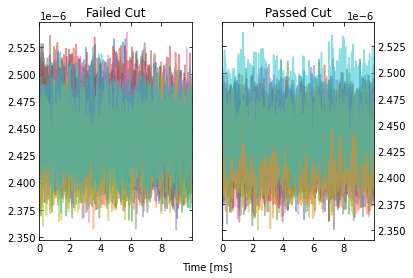
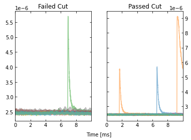
IC = IterCut(traces, fs, plotall=True)
cmaximum = IC.arbitrarycut(maximum, 200, cut=2)
cpileup = IC.pileupcut(cut=2)
cslope = IC.slopecut(cut=2)
cut_ic = IC.cmask
print(f"The maximum cut efficiency is {np.sum(cmaximum)/len(traces):.3f}.")
print(f"The pileup cut efficiency is {np.sum(cpileup)/np.sum(cmaximum):.3f}.")
print(f"The slope cut efficiency is {np.sum(cslope)/np.sum(cpileup):.3f}.")
print("-------------")
print(f"The total cut efficiency is {np.sum(cut_ic)/len(traces):.3f}.")
The maximum cut efficiency is 0.721.
The pileup cut efficiency is 0.742.
The slope cut efficiency is 0.763.
-------------
The total cut efficiency is 0.408.
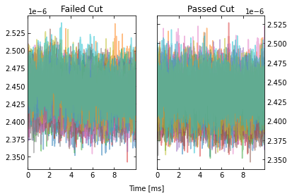
Looking at the events that passed, we see that the maximum cut we applied allowed a “bad” trace (a trace with a pulse). This makes sense since we only looked at a portion of the trace for that cut, so it was not a very good cut. Fortunately, our pileup and slope cuts did a good job of removing the bad traces that passed the maximum cut.
Lastly, it’s worth simply printing out the docstrings of the three
different supported outlier algorithms. The kwargs vary considerably
between each of them, so to specify them in IterCut, one must know
which ones to use! For example, iterstat has the cut kwarg,
which we were using in the above examples (because iterstat is the
default outlier algorithm for these automated cut routines).
from qetpy.cut import iterstat, removeoutliers
from astropy.stats import sigma_clip
?iterstat
Function to iteratively remove outliers based on how many standard
deviations they are from the mean, where the mean and standard
deviation are recalculated after each cut.

Parameters
----------
data : ndarray
    Array of data that we want to remove outliers from.
cut : float, optional
    Number of standard deviations from the mean to be used for
    outlier rejection
precision : float, optional
    Threshold for change in mean or standard deviation such that we
    stop iterating. The threshold is determined by
    np.std(data)/precision. This means that a higher number for
    precision means a lower threshold (i.e. more iterations).
return_unbiased_estimates : bool, optional
    Boolean flag for whether or not to return the biased or
    unbiased estimates of the mean and standard deviation of the
    data. Default is False.

Returns
-------
datamean : float
    Mean of the data after outliers have been removed.
datastd : float
    Standard deviation of the data after outliers have been
    removed.
datamask : ndarray
    Boolean array indicating which values to keep or reject in
    data, same length as data.
?removeoutliers
Function to return indices of inlying points, removing points
by minimizing the skewness.

Parameters
----------
x : ndarray
    Array of real-valued variables from which to remove outliers.
maxiter : float, optional
    Maximum number of iterations to continue to minimize skewness.
    Default is 20.
skewtarget : float, optional
    Desired residual skewness of distribution. Default is 0.05.

Returns
-------
inds : ndarray
    Boolean indices indicating which values to select/reject, same
    length as x.
?sigma_clip
Perform sigma-clipping on the provided data.

The data will be iterated over, each time rejecting values that are
less or more than a specified number of standard deviations from a
center value.

Clipped (rejected) pixels are those where::

    data < center - (sigma_lower * std)
    data > center + (sigma_upper * std)

where::

    center = cenfunc(data [, axis=])
    std = stdfunc(data [, axis=])

Invalid data values (i.e., NaN or inf) are automatically clipped.

For an object-oriented interface to sigma clipping, see
SigmaClip.

.. note::
    scipy.stats.sigmaclip provides a subset of the functionality
    in this class. Also, its input data cannot be a masked array
    and it does not handle data that contains invalid values (i.e.,
    NaN or inf). Also note that it uses the mean as the centering
    function. The equivalent settings to scipy.stats.sigmaclip
    are::

        sigma_clip(sigma=4., cenfunc='mean', maxiters=None, axis=None,
        ...        masked=False, return_bounds=True)

Parameters
----------
data : array-like or ~numpy.ma.MaskedArray
    The data to be sigma clipped.

sigma : float, optional
    The number of standard deviations to use for both the lower
    and upper clipping limit. These limits are overridden by
    sigma_lower and sigma_upper, if input. The default is 3.

sigma_lower : float or None, optional
    The number of standard deviations to use as the lower bound for
    the clipping limit. If None then the value of sigma is
    used. The default is None.

sigma_upper : float or None, optional
    The number of standard deviations to use as the upper bound for
    the clipping limit. If None then the value of sigma is
    used. The default is None.

maxiters : int or None, optional
    The maximum number of sigma-clipping iterations to perform or
    None to clip until convergence is achieved (i.e., iterate
    until the last iteration clips nothing). If convergence is
    achieved prior to maxiters iterations, the clipping
    iterations will stop. The default is 5.

cenfunc : {'median', 'mean'} or callable, optional
    The statistic or callable function/object used to compute
    the center value for the clipping. If using a callable
    function/object and the axis keyword is used, then it must
    be able to ignore NaNs (e.g., numpy.nanmean) and it must have
    an axis keyword to return an array with axis dimension(s)
    removed. The default is 'median'.

stdfunc : {'std', 'mad_std'} or callable, optional
    The statistic or callable function/object used to compute the
    standard deviation about the center value. If using a callable
    function/object and the axis keyword is used, then it must
    be able to ignore NaNs (e.g., numpy.nanstd) and it must have
    an axis keyword to return an array with axis dimension(s)
    removed. The default is 'std'.

axis : None or int or tuple of int, optional
    The axis or axes along which to sigma clip the data. If None,
    then the flattened data will be used. axis is passed to the
    cenfunc and stdfunc. The default is None.

masked : bool, optional
    If True, then a ~numpy.ma.MaskedArray is returned, where
    the mask is True for clipped values. If False, then a
    ~numpy.ndarray and the minimum and maximum clipping thresholds
    are returned. The default is True.

return_bounds : bool, optional
    If True, then the minimum and maximum clipping bounds are also
    returned.

copy : bool, optional
    If True, then the data array will be copied. If False
    and masked=True, then the returned masked array data will
    contain the same array as the input data (if data is a
    ~numpy.ndarray or ~numpy.ma.MaskedArray). If False and
    masked=False, the input data is modified in-place. The
    default is True.

grow : float or False, optional
    Radius within which to mask the neighbouring pixels of those
    that fall outwith the clipping limits (only applied along
    axis, if specified). As an example, for a 2D image a value
    of 1 will mask the nearest pixels in a cross pattern around each
    deviant pixel, while 1.5 will also reject the nearest diagonal
    neighbours and so on.

Returns
-------
result : array-like
    If masked=True, then a ~numpy.ma.MaskedArray is returned,
    where the mask is True for clipped values and where the input
    mask was True.

    If masked=False, then a ~numpy.ndarray is returned.

    If return_bounds=True, then in addition to the masked array
    or array above, the minimum and maximum clipping bounds are
    returned.

    If masked=False and axis=None, then the output array
    is a flattened 1D ~numpy.ndarray where the clipped values
    have been removed. If return_bounds=True then the returned
    minimum and maximum thresholds are scalars.

    If masked=False and axis is specified, then the output
    ~numpy.ndarray will have the same shape as the input data
    and contain np.nan where values were clipped. If the input
    data was a masked array, then the output ~numpy.ndarray
    will also contain np.nan where the input mask was True.
    If return_bounds=True then the returned minimum and maximum
    clipping thresholds will be be ~numpy.ndarrays.

See Also
--------
SigmaClip, sigma_clipped_stats

Notes
-----
The best performance will typically be obtained by setting
cenfunc and stdfunc to one of the built-in functions
specified as as string. If one of the options is set to a string
while the other has a custom callable, you may in some cases see
better performance if you have the `bottleneck`_ package installed.

.. _bottleneck:  https://github.com/pydata/bottleneck

Examples
--------
This example uses a data array of random variates from a Gaussian
distribution. We clip all points that are more than 2 sample
standard deviations from the median. The result is a masked array,
where the mask is True for clipped data::

    >>> from astropy.stats import sigma_clip
    >>> from numpy.random import randn
    >>> randvar = randn(10000)
    >>> filtered_data = sigma_clip(randvar, sigma=2, maxiters=5)

This example clips all points that are more than 3 sigma relative
to the sample mean, clips until convergence, returns an unmasked
~numpy.ndarray, and does not copy the data::

    >>> from astropy.stats import sigma_clip
    >>> from numpy.random import randn
    >>> from numpy import mean
    >>> randvar = randn(10000)
    >>> filtered_data = sigma_clip(randvar, sigma=3, maxiters=None,
    ...                            cenfunc=mean, masked=False, copy=False)

This example sigma clips along one axis::

    >>> from astropy.stats import sigma_clip
    >>> from numpy.random import normal
    >>> from numpy import arange, diag, ones
    >>> data = arange(5) + normal(0., 0.05, (5, 5)) + diag(ones(5))
    >>> filtered_data = sigma_clip(data, sigma=2.3, axis=0)

Note that along the other axis, no points would be clipped, as the
standard deviation is higher.